(Draft)Dynamics Of Legged Robots
Floating Base Systems
This post elaborates the dynamics of a floating base system that makes and breaks contact with the environment. In this post specifically we model the dynamics of a quadruped.
In general any system that can move in the environment is a floating base system, for a floating base system the generalized co-ordinates are modified to include the floating base position and orientation, in a quadruped it is usually the torso. The system is then described by by \(n_b\) un-actuated base coordinates \(q_b\) and \(n_j\) actuated joint coordinates \(q_j\)
\[\mathbf{q} = \begin{pmatrix} \mathbf{q_b} \\ \mathbf{q_j} \end{pmatrix}\] \[\mathbf{q_b} = \begin{pmatrix} \mathbf{q_{bP}} \\ \mathbf{q_{bR}} \end{pmatrix}\tag{2}\]The position \(\mathbf{q_{bP}}\) and rotation \(\mathbf{q_{bR}}\) can be parameterized using different representations. In this post I will be using exponential coordinates. For more information please refer to Lecture Notes on Robot Dynamics1 from which most of this article borrows from.
The generalized velocity \(\mathbf{u}\) and acceleration \(\dot{\mathbf{u}}\) is described by
\[\mathbf{u} = \begin{pmatrix} ^I\mathbf{v}_B \\ ^B\boldsymbol{\omega}_{IB} \\ \dot{\varphi}_1 \\ \vdots \\ \dot{\varphi}_{n_j} \end{pmatrix} \in \mathbb{R}^{6+n_j} = \mathbb{R}^{n_u}, \quad \dot{\mathbf{u}} = \begin{pmatrix} ^I\dot{\mathbf{v}}_B \\ ^B\dot{\boldsymbol{\omega}}_{IB} \\ \ddot{\varphi}_1 \\ \vdots \\ \ddot{\varphi}_{n_j} \end{pmatrix} \in \mathbb{R}^{6+n_j} \tag{2.245}\]Friction Cone
In the Coloumb Friction model, a static object that is in contact with the ground is associated with a friction force when an external force is applied on the body. This force is proportional to the Normal Force - \(\mathbf{\lambda_n}\) the proportionality constant is called the Friction coefficient \(\mu\).
If a body is stable and unmoving when the external force is applied it is assumed to be localized in a friction cone
\[\mathbf{\lambda_c} \leq \mu \mathbf{\lambda_n}\] \[\mathbf{\lambda_{ct}}^2 + \mathbf{\lambda_{cn}}^2 \leq \mu^2\mathbf{\lambda_n}^2\]where \(\mathbf{\lambda_{ct}}, \mathbf{\lambda_{cn}}\) are the tangential and normal components respectively. This paper2 proposes a linearized friction cone model which is
\[\mu\mathbf{\lambda_n} + |\mathbf{\lambda_{ct}}| \geq 0\] \[\mu\mathbf{\lambda_n} + |\mathbf{\lambda_{cn}}| \geq 0\]where |.| is the absolute value operator.
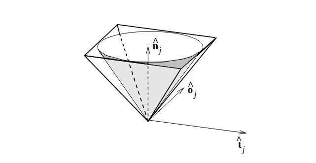 The friction cone with components \(\mathbf{n}\) - normal and the two tangential components \(\mathbf{t},\mathbf{o}\) subscript \(\mathbf{j}\) is the index of the contact and the super script ^ indicates a unit vector 2
Dynamics
\[\mathbf{M}(\mathbf{q}) \ddot{\mathbf{q}}+\mathbf{C}(\mathbf{q}, \mathbf{\dot q})+\mathbf{G}(\mathbf{q})=\mathbf{S}^T \boldsymbol{\tau}+\mathbf{J}_{e x t}^T \mathbf{F}_{e x t}\]consisting of the following components:
| Symbol | Dimension | Description |
|---|---|---|
| \(\mathbf{M}(\mathbf{q})\) | \(\in \mathbb{R}^{n_q \times n_q}\) | Mass matrix (orthogonal) |
| \(\mathbf{q}\) | \(\in \mathbb{R}^{n_q}\) | generalized coordinates |
| \(\ddot{\mathbf{q}}\) | generalized acceleration | |
| \(\mathbf{C}(\mathbf{q}, \mathbf{\dot q})\) | \(\in \mathbb{R}^{n_q}\) | Coriolis and centrifugal terms |
| \(\mathrm{G}(\mathbf{q})\) | \(\in \mathbb{R}^{n_q}\) | gravitational terms |
| \(\mathbf{S}\) | \(\in \mathbb{R}^{n_\tau \times n_q}\) | selection matrix of actuated joints |
| \(\boldsymbol{\tau}\) | \(\in \mathbb{R}^{n_\tau}\) | generalized torques acting in direction of generalized coordinates |
| \(\mathbf{F}_{\text{ext}}\) | \(\in \mathbb{R}^{n_c}\) | external forces acting |
| \(\mathbf{J}_{\text{ext}}\) | \(\in \mathbb{R}^{n_c \times n_q}\) | (geometric) Jacobian of location where external forces apply |
the derivation of these terms can be found in the lecture notes1
Control
In this post I will be following the control method described in this paper3. The control problem is formulated as LCP (Linear Complementarity Problem) which is a convex optimization problem. The LCP is formulated as follows:
\[\begin{equation} \begin{array}{ll} \text { find } & \ddot{q}, \lambda \\ \text { subject to } & M(q) \ddot{q}+C(q, \dot{q})+G(q)=B(q) u+J(q)^{\mathrm{T}} \lambda \\ & \phi(q) \geq 0 \\ & \lambda \geq 0 \\ & \phi(q)^{\mathrm{T}} \lambda=0 \end{array} \end{equation}\]where \(\phi(q)\) is the non-penetration constraint(example: Signed Distance Field), indicating if the robot made contact with the environment, \(\lambda\) is the contact force, \(B(q)\) is the control input matrix, \(J(q)\) represents the Jacobian projecting constraint forces into the generalized coordinates \(J(q) = \frac{\partial\phi(q)}{\partial q}\) , \(M(q)\) is the joint-space inertia matrix, \(C(q,\dot{q})\) is the Coriolis and centrifugal terms, \(G(q)\) is the gravitational terms.
Trajectory Optimization Approach
Rather than solving the control problem directly, which involves solving for the contact force \(\lambda\) at each time step. The paper proposes to optimize over the space of feasible states, control inputs, constraint forces, and trajectory durations, while treating the contact forces as optimization variables.With \(g( ·, ·)\) and \(g_f (·)\) being the integrated and final cost functions respectively, the optimization problem can be written as follows:
\[\begin{equation} \underset{\left\{h_x, \ldots, x_N, u_1, \ldots, u_N, \lambda_1, \ldots, \lambda_N\right\}}{\operatorname{minimize}} g_f\left(x_N\right)+h \sum_{k=1}^N g\left(x_{k-1}, u_k\right) \end{equation}\]References
Robot Dynamics Lecture Notes. Robotic Systems Lab, ETH Zurich, HS 2017. ↩︎ ↩︎2
On Dynamic Multi-Rigid-Body Contact Problems with Coulomb Friction. Trinkle, J.C., Pang, J.S., and Sandra, S., Grace, Lo. September 1985 ↩︎ ↩︎2
A Direct Method for Trajectory Optimization of Rigid Bodies Through Contact. Michael Posa, Cecilia Cantu and Russ Tedrake. 2013 ↩︎